Challenge accepted.

What I’m trying to achieve

Get oriented in this project, get the repo up, get the log started on meej.ca, learn about the space. This is my first RL project and I come from a CV/IL background so this will be hard.

Thoughts

I need to learn and ship this project fast. As a result, my approach will be to de-scope as much as possible. The question is what makes a solution to this challenge more creative than another? There are a few approaches to take:

1. The solution has a truly great implementation of RL: punching above your weight (for your education/age) is a fantastic way to show intuition and creativity.
2. The solution has a unique behaviour: whether it be something quirky or useful, coming up with a unique solution to a simple problem is almost by definition a creative approach.
3. The content of your presentation is communicated clearly, concisely, and in a way that is visually appealing: engineering is not just about creating the product, it’s also about creating a way to communicate what you’ve done elegantly.

For this 11-day challenge, my goal is to launch a 3D End-Effector Tracking Arm and communicate each step of the way in a way that’s easy to follow. I will demonstrate the difference between an RL solution and a standard inverse kinematics / PI control solution, with some commentary on both approaches.

Research

To de-scope, I have to ask whether the documentation around the Franka arm (7DoF) is a greater advantage over the fewer dimensions of the UR5 arm (6DoF).

Franka Panda is the de facto default for RL manipulation research, which means dozens of public Gymnasium environments, SB3 examples, reward functions, and obs designs you can crib from. UR5 has more industrial-automation code and less RL-flavored code. The 7th DoF on Franka is also irrelevant at the RL level if we use a Cartesian action space

(the wrapper handles inverse kinematics under the hood, agent never sees joints).

After researching the space a little more with the help of Claude, it makes sense to go with the option with more documentation, especially considering the extra dimension will get baked into our reward system anyway.

The next natural question is: do we care about the orientation of the tip of the arm? We want to ship fast, so we can de-scope the problem to ignore the orientation of the tip of the arm and focus on position only.

What is the action space of the RL model?

Well, it’s baked into the problem description. It should naturally be the cartesian end-effector delta. This means we don’t care about the arm joints, we just care about the final position of the tip, and the model picks how it will move the joints.

What will the reward shape look like?

A standard shape: ||target - current_ee|| - α·||action||, that second term is a magnitude penalty for smoothness which we can tune later.

What will our observations look like?

The set of {ee_pos, ee_vel, target_pos, target_vel, error}. Keep it simple for now. The idea is the arm needs to see where it is and where it’s going to go.

What will the RL algo look like?

PPO via SB3, not from scratch… I’ve heard about these two tools in passing, so it will be a delight to learn more about them as we go along.

Experiment

Going through the motions

I’m going to need a virtual environment to do any development, luckily I just downloaded uv for a course at UBC (CPSC 330, intro to ML). I can reuse it here to make a new environment for this project.

uv init rl-arm-tracking in my /Projects directory will do the trick (I’ve also added a description). Ok, now we can update the README.md a little, delete the useless main.py for now, and launch the repo using the GitHub CLI: github.com/amjadya/rl-arm-tracking, boom.

Some dependencies

uv add mujoco numpy matplotlib robot_descriptions

• mujoco: gives us the physics engine we need
• numpy: classic array math… MuJoCo state is numpy arrays!
• matplotlib: hehe, plots
• robot_descriptions: this is a community package with a bunch of MJCF/URDF files (Franka is in there)

The first script

import mujoco
import mujoco.viewer
from robot_descriptions import panda_mj_description


def main() -> None:
    model = mujoco.MjModel.from_xml_path(panda_mj_description.MJCF_PATH)
    data = mujoco.MjData(model)

    mujoco.viewer.launch(model, data)

if __name__ == "__main__":
    main()

Why two objects? One has the topology of the Franka arm we have access to through the robot_descriptions package, and MjData holds the arm’s state.

	MjModel	MjData
What	Fixed blueprint	Current state
Mutates?	No, ever	Yes, every step
Created via	XML parsing	Memory allocation sized to model
How many	Usually one	Can have many, all sharing the same model

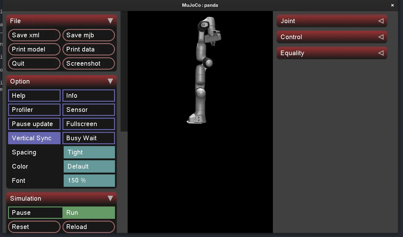
Running uv run python hello_arm.py gives us the following:

A note on the API asymmetry

MjModel.from_xml_path(...) is a factory method because there are multiple ways a model can come into existence (XML file, XML string, compiled binary). The canonical creation path is “parse this XML file.” Hence the named constructor.

MjData(model) is just allocating zeroed-out buffers sized to the model. There’s no parsing involved. MuJoCo looks at model.nq, model.nv, model.nu, etc., and allocates arrays of that size. So a plain constructor with (model) as the size hint is all that’s needed.

Why this matters for our RL pipeline: when we vectorize training (run many parallel envs to feed the policy), we’ll likely have one MjModel (loaded once, slow-ish) and many MjData objects (one per env, cheap to allocate).

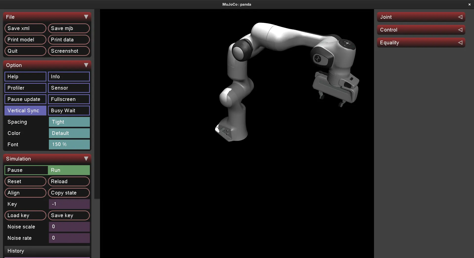
XML keyframe

mujoco.mj_resetDataKeyframe(model, data, 0) gives the arm a more natural pose.

Getting familiar with the Franka robot arm

Let’s print some important features to the terminal so we know what we’re working with:

Model: /home/meej/.cache/robot_descriptions/mujoco_menagerie/franka_emika_panda/panda.xml

njnt = 9 (joints)
nq = 9 (generalized coordinates)
nv = 9 (degrees of freedom)
nu = 8 (actuators)
nbody = 12

Joints:
[0] joint1
[1] joint2
[2] joint3
[3] joint4
[4] joint5
[5] joint6
[6] joint7
[7] finger_joint1
[8] finger_joint2

Actuators:
[0] actuator1
[1] actuator2
[2] actuator3
[3] actuator4
[4] actuator5
[5] actuator6
[6] actuator7
[7] actuator8

Nine joints, eight actuators… interesting. It seems that on a real Franka gripper, the two finger joints are actuated together. Good to know. We don’t really care for this as we won’t be using the gripper for the end-effector trajectory tracking.

Also note, MuJoCo is exposing generalized coords AND degrees of freedom. This is scary because it implies we’re going to have to worry about quaternions. Flagging this as something to learn more about if issues come up. (Hopefully my Lagrangian mechanics course can help out here…)

Driving questions

• What position should I leave the gripper in?
• To what extent will I have to revisit quaternions in order to simulate the arm physics correctly?
• Does the chosen reward shape ||target − ee|| − α·||action|| actually produce smooth motion, or will it need extra terms (per-axis weighting, derivative)?

Next

• Write a script that drives the arm’s end-effector to a hardcoded 3D point in space using iterative inverse kinematics (Jacobian pseudo-inverse). This is the foundation that gets reused twice: as part of the RL env’s Cartesian action wrapper, and as the classical IK+PD baseline.