Wiring the RL pipeline end-to-end

What I’m trying to achieve

Today’s goal is to close out trajectory.py, build the three remaining pipeline files (env.py, train.py, eval.py), train a first policy on the new infrastructure, and watch it run.

Research

I have to get stronger with the terminology if I’m going to build anything useful. Here are the definitions in my own words.

Markov Decision Process vocabulary

• Observation space: the schema for the agent’s inputs.
• Observation: the current values seen by the agent.
• State: the complete state of the system, whether or not the agent can see it.
• Action: the agent’s output. In our case, a Cartesian vector we call “lead”.
• Reward: the equation that promotes good behaviour and punishes bad behaviour.
• Episode: one full run from start to termination.
• Transition: a single step of the simulation, written as (s, a, r, s'). “I was in state s, took action a, got reward r, and ended up in next-state s’.”
• Return: the total reward across all transitions in an episode.
• Discount: reduces the impact later rewards have on return, and mathematically bounds the total reward for long episodes.

Gymnasium API

Gymnasium is a thin interface that separates the RL algorithm from the environment. To make a custom env, I declare or implement:

1. self.observation_space and self.action_space in __init__.
2. reset(): starts a fresh episode. Puts the environment back in a valid starting state and returns the first observation. By the time reset() is called, the previous episode is already done; it just waits to be reborn.
3. step(action): advances one transition. Returns (obs, reward, terminated, truncated, info).

That contract is the whole interface SB3’s PPO needs to talk to my env.

Space: the shape of valid data. The most common is Box:

from gymnasium.spaces import Box
import numpy as np

# A 3D vector where each component is in [-1, 1]
some_space = Box(low=-1.0, high=1.0, shape=(3,), dtype=np.float32)

The shape is what matters most. For observation_space, the bounds are mostly informational (SB3 does not clip observations to them). For action_space, the bounds are enforced: the policy’s outputs are clipped to that range.

PPO concepts

• Policy: the network that makes decisions. The policy returns a probability distribution over actions. Call it twice on the same observation and you get a different result.

• Value function: a second network that estimates the expected total discounted return from a given state. PPO is an “actor-critic” method: the policy is the actor (picks actions), the value function is the critic (judges states). The value function provides the baseline used to compute advantage, and trains itself separately to predict returns more accurately.

• Advantage: the difference between what actually happened and what the value function predicted. advantage = G − V(s). This is the interesting part of what happened in the episode (better or worse than expected). PPO uses positive advantage to encourage actions and negative advantage to discourage them.

• Rollout: a batch of transitions collected from running the policy. PPO collects a rollout, computes advantages, runs several gradient updates on it, then throws it away and collects fresh data. Contents:

Stored	Needed for
observation s	feeding through policy + value nets
action a	knowing what was tried
reward r	computing return / advantage
log_prob of a	the PPO loss formula
value estimate V(s)	computing advantage

The size of the rollout is a hyperparameter; SB3’s PPO default is 2048 per env.

• On-policy: an algorithm that can only train on data collected by the current policy. Once the weights shift, the stored rollout no longer reflects current behaviour and has to be discarded.

Experiment

trajectory.py

Picking up where last session left off, I started simple: randomly generated circular trajectories with different centre positions and orientations.

uv run trajectory.py --show --seed 0

uv run trajectory.py --show --seed 10

Something to think about: what happens when the trajectory passes through the arm’s own body? I’ll defer this and treat it as an “unreachable position” for now.

See trajectory.py on GitHub.

env.py

Two flags I had to internalise:

• Terminated: the episode ended because of a failure or success condition.
• Truncated: the episode ran out of time (max steps exceeded).

Two design choices that don’t have a “right” answer:

• How many steps per episode? By choice: enough to see at least one full trajectory loop. I picked 200.
• How often should the policy make decisions? By choice: slower than the physics loop (500 Hz), faster than a human could react. I picked 100 Hz, giving 5 physics ticks per control tick.

The rest of env.py fell out naturally once the MDP, Gymnasium, and PPO concepts above were settled. See env.py on GitHub.

train.py

The plan for this file:

1. Build vectorised envs.
2. Construct the PPO model.
3. Set up callbacks for logging and evaluation against a validation set.
4. Run training (model.learn()).

Vec env shape: I have 16 cores, so technically I could go up to 16. Since I don’t know how to set up scheduling yet, I started with 8 and left room to scale.

A few concepts that fell out of building this:

• SubprocVecEnv spawns 8 new Python processes, each with its own memory, variables, and imports. To run make_env inside a subprocess, the subprocess imports the module that defines the env. In our case, that’s train.py itself.
• if __name__ == "__main__": is what stops the multiprocessing from re-spawning subprocesses on import and blowing the OS up.
• The factory pattern (make_env()) is needed because MuJoCo’s C pointers can’t be pickled. We can’t ship a pre-built env to a subprocess, but we can ship a function that builds one locally.

PPO hyperparameters

Argument	Value	Meaning
"MlpPolicy"	—	Default MLP (two hidden layers of 64 units, tanh activations). Gives us mean, log-std, and value heads.
vec_env	—	The parallel envs PPO will sample from.
seed	42	PPO’s internal RNG. Not related to the env seed.
n_steps	1024	Steps per env per rollout.
batch_size	64	Mini-batch size inside the gradient update.
n_epochs	10	Passes over the rollout per update (n_envs * n_steps / batch_size = 128 mini-batches per epoch).
gamma	0.99	Discount factor. Bounds the infinite-horizon return and sets the agent’s effective planning horizon.
gae_lambda	0.95	Blend between Monte Carlo and bootstrap when estimating G for advantage. Closer to 1 leans Monte Carlo.
learning_rate	3e-4	Scales Adam (PPO’s optimiser) to control the size of each weight update.
clip_range	0.2	Hard limit on how much the policy can shift in a single gradient update.
ent_coef	0.0	Entropy pressure. Rewards the policy for staying exploratory. Tune up if it commits to local optima too early.

Callbacks

Two callbacks for logging and saving the best-seen model:

• CheckpointCallback: periodic full-model snapshots to ./checkpoints/. Crash insurance.
• EvalCallback: validates the current policy against five deterministic episodes in a separate env (clean of the eight training subprocesses), and saves the best-performing checkpoint to ./checkpoints/best/.

The eval fires five times more often than checkpointing: roughly every six rollouts I save weights, but I validate the policy almost every rollout.

Training run

And that’s it. I set TOTAL_TIMESTEPS = 1_000_000, added tensorboard_log="./logs/tb/" to the PPO constructor, and pulled in the extras:

uv add tqdm rich tensorboard

Through a conversation with Claude, I learned that tensorboard_log is one way to capture the metrics that diagnose training health:

• train/policy_loss: is the policy actually being pushed by gradients?
• train/value_loss: is V(s) getting better at predicting G?
• train/entropy_loss: how spread out is the policy?
• train/approx_kl: how much did the policy shift per update?
• train/clip_fraction: what % of transitions hit the clip_range cap?
• train/explained_variance: how well does V(s) explain the actual returns? (~1 = great, ~0 = useless).
• rollout/ep_rew_mean: mean training reward (noisy, exploratory).

A smoke test at TOTAL_TIMESTEPS = 10_000 flagged a warning that PPO with an MLP policy runs faster on CPU than GPU, so I added device="cpu" to the PPO constructor.

After suppressing the minor warnings:

uv run python train.py
uv run tensorboard --logdir ./logs/

It took 17 minutes.

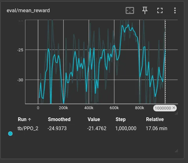
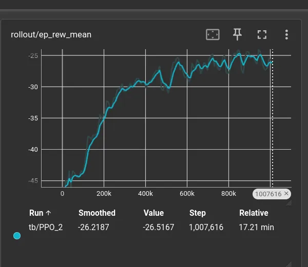
Not bad: the smoothed rollout/ep_rew_mean climbs from -45 to roughly -25 and plateaus around step 500k. The eval/mean_reward is noisier (only five episodes per evaluation), but reaches a best of -17.16 ± 3.02 at step 660,000 before settling at -21.48 ± 6.95 by the end. Whether this is a local minimum or the physical floor of the task is the next thing I want to investigate visually.

See train.py on GitHub.

eval.py

Only a few lines, and largely similar to work we’ve done before. See eval.py on GitHub.

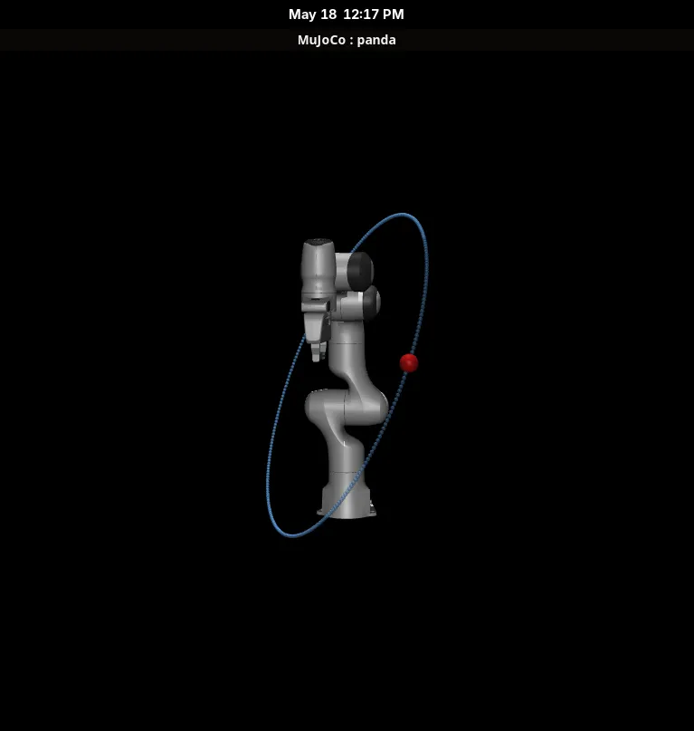
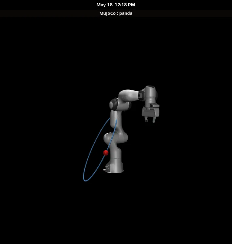
Otherwise, here’s a video of its performance:

Even on just 1M steps the feed-forward is visibly learned.

The arm hits itself occasionally. I don’t know yet whether this is the RL or the IK; I’ll need to compare trajectories across the classical and RL controllers before drawing a conclusion. My suspicion is it’s IK, not RL.

Two paths to fix it: add a collision penalty to the reward (which would improve RL tracking over the classical approach even more), or bias the IK toward solutions less likely to self-collide.

At this stage, I’m ready to add an offset to the end-effector so we can see it tracking the red ball without the wrist mesh clipping over the visualisation.

Driving questions

• How do I get the arm to stop hitting itself? Collision penalty in the reward, or IK bias toward less-collision-prone configurations?
• How do I make sure I compare apples to apples between the classical and RL controllers, given the agent acts at 100 Hz while IK+PD ran as fast as the physics loop (500 Hz)?
• Is max_lead = 0.15 m valid given my assumption that trajectories won’t exceed 2.5 m/s? When does that break?
• What trajectory shapes should I train on next, and in what mix? Only circles so far.

Next

• Compare the feed-forward-trained policy against the classical IK + PD controller from the May 15 entry.
• Move the tracked end-effector point to an offset past the wrist so tracking is visible without the wrist mesh clipping the marker. Note: this changes the EE definition and will require retraining.